How To Download ArcGis Data For Halifax Using R

In this post, how to download data directly for the public datasets for Halifax are demonstrated for R

Introduction

Halifax Municipality provides access to a range of data sets via ArcGis.

The full catalog of data is available here:

https://catalogue-hrm.opendata.arcgis.com/

In this blog post, we will cover how to download this data into R for further analysis.

For this example, we will be using the Crime Dataset which details the past 7 days of crime in HRM.

Locate Dataset API URL

Fig 1.

First, we need to locate the data set we want to use on the Halifax open data webpage.

Once you’ve found a dataset you would like to use:

1. Click I want to use this
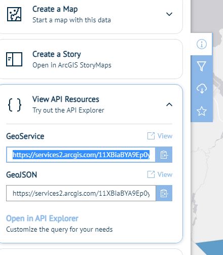
2. Click View API Resources
3. Copy the provided link from GeoService (Fig 1.)

The url obtained in step 3 is what we will use to access the data. The URL can be modified to include query information, and the result will be a dataset in JSON format which we can then parse for data.

Creating The Function

The next step is to create a function that downloads the data from the data_url.

However, one limitation is that the API only allows us to download up to 2000 rows at a time. This likely won’t be an issue for this particular data set as it’s currently only ~100 rows, however, just to be safe for future issues, we will use a recursive method so that the function will call itself to download additional data until it find no additional records..

Here’s an example of the code for this function:

#' Download arcgis data
#'
#' This function will download all data for a given URL
#'
#' @data_url the url of the resource from arcGis
#' @result_offset The offset to be added when returning the results; typically this should be left as 0; the function will changes this value as needed to pull additional results
arcGis_getData <- function(data_url = NULL, result_offset = 0){
  
  #Get the data for the given data_url and result_offset
  query_response <- httr::GET(data_url,
                        query = list(resultOffset=result_offset))
  
  #Checks for errors produced by the request
  httr::stop_for_status(query_response)
  
  #Obtains the json results from the response
  results_json <- jsonlite::fromJSON(rawToChar(query_response$content))
  
  #Determines if there are more results based off the existence of the exceedTransferLimit as well as it being TRUE
  more_results <- ifelse(is.null(results_json$exceededTransferLimit), FALSE, results_json$exceededTransferLimit)
  
  #Returns the results from the request
  results_data <- results_json$features$attributes
  
  #Checks if the data set has geometry, and adds to the results if true
  Data_Geo <- results_json$features$geometry
  results_data <- dplyr::bind_cols(results_data, Data_Geo)
  
  
  #If there were more results, the function is called recursively and the data is added to the results
  if(more_results){
    results_data <- data.table::rbindlist(list(results_data,
                                          arcGis_getData(
                                            data_url,
                                            result_offset = result_offset + 2000)))
  }
  
  #Returns the final dataset
  results_data
}

Using The Function

To use this function, we need to provide it with the data_url for the data set we want to download. In this case, the data_url for the Crime dataset is:

https://services2.arcgis.com/11XBiaBYA9Ep0yNJ/arcgis/rest/services/Crime/FeatureServer/0/query?where=1%3D1&outFields=*&outSR=4326&f=json

We then call the function using this data_url:

#URL for the data
Query_URL <- 'https://services2.arcgis.com/11XBiaBYA9Ep0yNJ/arcgis/rest/services/Crime/FeatureServer/0/query?where=1%3D1&outFields=*&outSR=4326&f=json'

#Get the data
all_data <- arcGis_getData(Query_URL)

The result will be a data frame containing all the data from the data set:

head(all_data)

  ObjectID evt_rt evt_rin     evt_date        location rucr         rucr_ext_d
1        1     GO 1273815 1.678421e+12        DAVIS DR 1430            ASSAULT
2        2     GO 1273918 1.678421e+12 LADY HAMMOND RD 2120    BREAK AND ENTER
3        3     GO 1273768 1.678421e+12       MORRIS ST 2142 THEFT FROM VEHICLE
4        4     GO 1273856 1.678421e+12     BEDFORD HWY 2135   THEFT OF VEHICLE
5        5     GO 1273805 1.678421e+12  TERRADORE LANE 1430            ASSAULT
6        6     GO 1273787 1.678421e+12   FALL RIVER RD 1420            ASSAULT
          x        y
1 -63.68747 44.86725
2 -63.61402 44.66607
3 -63.57804 44.64002
4 -63.66148 44.70228
5 -63.73309 44.71334
6 -63.61630 44.81594

Looking at the data, we can see that the date in represented in UNIX time. This is common when using apis, but is easy to translate to a normal date format in R:

library(dplyr)

Warning: package 'dplyr' was built under R version 4.1.3

#Time is stored in UNIX epoch time; convert to POSIXct
all_data <- all_data %>%
  mutate(evt_date = as.Date(as.POSIXct(evt_date/1000, origin="1970-01-01")))

head(all_data)

  ObjectID evt_rt evt_rin   evt_date        location rucr         rucr_ext_d
1        1     GO 1273815 2023-03-10        DAVIS DR 1430            ASSAULT
2        2     GO 1273918 2023-03-10 LADY HAMMOND RD 2120    BREAK AND ENTER
3        3     GO 1273768 2023-03-10       MORRIS ST 2142 THEFT FROM VEHICLE
4        4     GO 1273856 2023-03-10     BEDFORD HWY 2135   THEFT OF VEHICLE
5        5     GO 1273805 2023-03-10  TERRADORE LANE 1430            ASSAULT
6        6     GO 1273787 2023-03-10   FALL RIVER RD 1420            ASSAULT
          x        y
1 -63.68747 44.86725
2 -63.61402 44.66607
3 -63.57804 44.64002
4 -63.66148 44.70228
5 -63.73309 44.71334
6 -63.61630 44.81594

Looks much better now!

Plotting Of The Data

One limitation of the map provided by the city is that they only provided data points.

Now that we have the data, we will cluster the crimes by location, and provide color coding of the crime type at higher resolutions.

library(leaflet)

Warning: package 'leaflet' was built under R version 4.1.3

pal <- colorFactor(
  palette = 'viridis',
  domain = all_data$rucr_ext_d
)

all_data %>%
  rowwise() %>%
  mutate(popup = paste0('Date: ', evt_date, '<br>', 'Location: ', location, '<br>', 'Crime: ', rucr_ext_d)) %>%
  leaflet() %>%
  addTiles() %>%
  addCircleMarkers(~x, ~y,
                   radius = 10,
                   clusterOptions = markerClusterOptions(),
                   popup = ~popup, 
                   color = ~pal(rucr_ext_d),
                   fillOpacity = .1) %>%
  addLegend(position = "bottomright", pal = pal, values = ~rucr_ext_d,
            title = "Crime")